Choosing the right counterfactual: ITS vs. synthetic control on the same data#
Here is one dataset. It has a clearly treated unit and seven unaffected controls. We will estimate the causal effect three ways — Google’s CausalImpact, CausalPy’s Interrupted Time Series, and CausalPy’s Synthetic Control — and the answers will differ by more than an order of magnitude. Understanding why tells us how to choose between ITS and synthetic control in general.
The short version of the lesson, which we will unpack below: when you have a donor pool of unaffected controls, modelling cross-unit structure beats extrapolating the treated unit’s own history. CausalImpact [] can take covariates and do CITS in principle, but when we put it on equal footing with a counterfactual built from the treated series alone — as we do here — the method’s failure mode reveals what ITS can and cannot answer.
Setup#
import warnings

warnings.filterwarnings("ignore")

import causalpy as cp
import arviz as az

import matplotlib.pyplot as plt
import seaborn as sns

import numpy as np
import pandas as pd

from causalimpact import CausalImpact
az.style.use("arviz-darkgrid")
plt.rcParams["figure.figsize"] = [10, 5]
plt.rcParams["figure.dpi"] = 100
plt.rcParams["axes.labelsize"] = 8
plt.rcParams["xtick.labelsize"] = 8
plt.rcParams["ytick.labelsize"] = 8
plt.rcParams.update({"figure.constrained_layout.use": True})

# Named semantic colours. Hue is tied to method *family* so the ITS-family
# methods share a colour family and synthetic control is visually distinct.
COLOR_CI = "#1f77b4"  # CausalImpact (ITS family, blue)
COLOR_ITS = "#4f9fd6"  # CausalPy ITS (ITS family, lighter blue)
COLOR_SC = "#d95f02"  # CausalPy Synthetic Control (distinct hue)

seed = sum(map(ord, "causalpy flexibility comparative"))
rng = np.random.default_rng(seed)
print(f"Seed: {seed}")
Seed: 3298
The Data: A Classic Synthetic Control Setting#
We’ll use CausalPy’s built-in sc dataset. This is a textbook scenario for Synthetic Control: one treated unit (actual) and seven control units (a through g) — the donor pool — observed over 100 time periods. The intervention happens at time 73.
df = cp.load_data("sc")
treatment_time = 73

control_units = ["a", "b", "c", "d", "e", "f", "g"]
treated_unit = "actual"

print(f"Shape: {df.shape}")
print(f"Columns: {df.columns.tolist()}")
print(f"Treatment time: {treatment_time}")
df.head()
Shape: (100, 10)
Columns: ['a', 'b', 'c', 'd', 'e', 'f', 'g', 'counterfactual', 'causal effect', 'actual']
Treatment time: 73
| a | b | c | d | e | f | g | counterfactual | causal effect | actual | |
|---|---|---|---|---|---|---|---|---|---|---|
| 0 | 0.793234 | 1.277264 | -0.055407 | -0.791535 | 1.075170 | 0.817384 | -2.607528 | 0.144888 | -0.0 | 0.398287 |
| 1 | 1.841898 | 1.185068 | -0.221424 | -1.430772 | 1.078303 | 0.890110 | -3.108099 | 0.601862 | -0.0 | 0.491644 |
| 2 | 2.867102 | 1.922957 | -0.153303 | -1.429027 | 1.432057 | 1.455499 | -3.149104 | 1.060285 | -0.0 | 1.232330 |
| 3 | 2.816255 | 2.424558 | 0.252894 | -1.260527 | 1.938960 | 2.088586 | -3.563201 | 1.520801 | -0.0 | 1.672995 |
| 4 | 3.865208 | 2.358650 | 0.311572 | -2.393438 | 1.977716 | 2.752152 | -3.515991 | 1.983661 | -0.0 | 1.775940 |
Let’s visualize what we’re working with. The treated unit lives among a family of control units — some trending up, some trending down, all moving through time together.
fig, ax = plt.subplots()
for i, col in enumerate(control_units):
    label = "Controls (a–g)" if i == 0 else None
    ax.plot(df.index, df[col], alpha=0.3, color="C0", linewidth=1, label=label)
ax.plot(df.index, df[treated_unit], color="black", linewidth=2, label="Treated unit")
ax.axvline(
    x=treatment_time, color="red", linestyle="--", linewidth=1.5, label="Intervention"
)
ax.set(
    title="Treated Unit Among Control Units",
    xlabel="Time",
    ylabel="Outcome",
)
ax.legend()
plt.show()
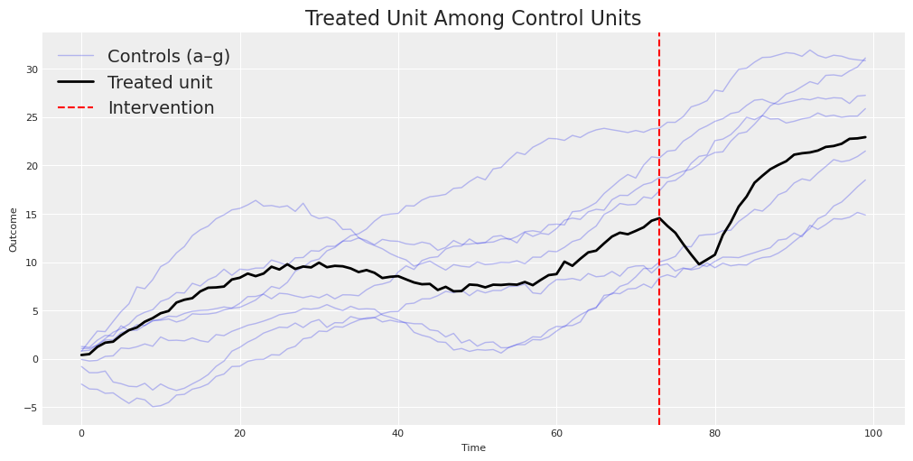
Notice the structure: the treated unit doesn’t just follow a smooth trend — it tracks a combination of the control units. After the intervention (the red dashed line), something changes. Our job is to estimate what changed and by how much — the causal effect.
This dataset is simulated with a known causal effect, so we can compare each method’s estimate to the true ATT over the post-intervention period. The simulated causal effect column averages to ≈ −1.85 over periods 73–99 — this is the simulation’s ATT over this window, not a fundamental property of the setup. Let’s see which method gets closest.
Attempt 1: Google’s CausalImpact (BSTS)#
Let’s start with the tool most people reach for: tfp-causalimpact, the Python port of Google’s CausalImpact []. This package uses a Bayesian Structural Time Series (BSTS) model to build a counterfactual from pre-intervention data and project it forward.
To keep this a fair comparison, we’ll give CausalImpact only the treated unit — no covariates. This puts it on equal footing with CausalPy’s ITS: both methods must build a counterfactual from the treated unit’s own time series alone. CausalImpact can accept control units as covariates (which would make it a CITS analysis); we leave that for the comparison that follows.
# Fair comparison: only the treated unit, no covariates
ci_data = df[[treated_unit]].copy()

pre_period = [0, treatment_time - 1]
post_period = [treatment_time, len(df) - 1]

ci = CausalImpact(ci_data, pre_period, post_period)
ci.plot()
plt.show()
print(ci.summary())
Posterior Inference {Causal Impact}
                          Average            Cumulative
Actual                    17.45              471.09
Prediction (s.d.)         8.15 (0.65)        220.01 (17.62)
95% CI                    [6.87, 9.43]       [185.59, 254.67]

Absolute effect (s.d.)    9.3 (0.65)         251.09 (17.62)
95% CI                    [8.02, 10.57]      [216.42, 285.51]

Relative effect (s.d.)    114.13% (8.01%)    114.13% (8.01%)
95% CI                    [98.37%, 129.77%]  [98.37%, 129.77%]

Posterior tail-area probability p: 0.0
Posterior prob. of a causal effect: 100.0%

For more details run the command: print(impact.summary('report'))
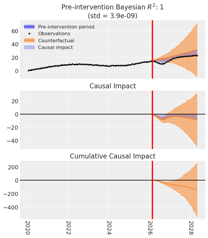
CausalImpact estimates an average effect of around +9.3 — the wrong sign, against a true effect near −1.85. With no access to the controls, the BSTS model must build a counterfactual from the treated series alone: it extrapolates the pre-period level and trend, and mis-attributes the post-period gap between treated unit and that extrapolation to the intervention. This is the expected failure mode of ITS when cross-sectional information is available but unused.
Let’s keep that in our pocket and see how CausalPy’s ITS does on the same single-series task.
Attempt 2: CausalPy’s ITS (State Space Model)#
Now let’s try the same ITS approach but using CausalPy’s structural state-space time-series model. CausalPy’s ITS is more transparent — we see the full Bayesian posterior and richer diagnostics — but the information it has access to is the same: the treated series and time.
A technical caveat before we fit: the state-space model expects a DatetimeIndex, so we attach an arbitrary monthly calendar to the integer time index. The seasonal_length=12 argument follows from that calendar and is not meaningful for this dataset — there is no real monthly seasonality to recover. The level and trend components do the real work here.
# ITS needs a time-indexed DataFrame with the outcome.
# NOTE: the monthly calendar here is arbitrary — the state-space model requires
# a DatetimeIndex, but the original dataset has an integer time index.
df_its = pd.DataFrame(
    {
        "y": df[treated_unit].values,
    },
    index=pd.date_range("2020-01-01", periods=len(df), freq="ME"),
)

its_treatment_time = df_its.index[treatment_time]
print(f"ITS treatment time: {its_treatment_time}")
df_its.head()
ITS treatment time: 2026-02-28 00:00:00
| y | |
|---|---|
| 2020-01-31 | 0.398287 |
| 2020-02-29 | 0.491644 |
| 2020-03-31 | 1.232330 |
| 2020-04-30 | 1.672995 |
| 2020-05-31 | 1.775940 |
sampler_kwargs = {
    "chains": 4,
    "draws": 550,
    "target_accept": 0.94,
    "random_seed": 42,
    "progressbar": False,
    "nut_sampler": "nutpie",
    "nuts_sampler_kwargs": {"backend": "jax", "gradient_backend": "jax"},
}

ssts_model = cp.pymc_models.StateSpaceTimeSeries(
    level_order=3,
    seasonal_length=12,
    sample_kwargs=sampler_kwargs,
    mode="FAST_COMPILE",
)

ssts_result = cp.InterruptedTimeSeries(
    df_its,
    its_treatment_time,
    formula="y ~ 1",
    model=ssts_model,
)
                                 Model Requirements

  Variable              Shape      Constraints                          Dimensions
 ──────────────────────────────────────────────────────────────────────────────────
  initial_level_trend   (3,)                                ('state_level_trend',)
  sigma_level_trend     (3,)       Positive                 ('shock_level_trend',)
  params_freq           (11,)                                      ('state_freq',)
  sigma_freq            ()         Positive                                   None
  P0                    (15, 15)   Positive semi-definite   ('state', 'state_aux')

These parameters should be assigned priors inside a PyMC model block before calling
                         the build_statespace_graph method.
Initializing NUTS using jitter+adapt_diag...
Multiprocess sampling (4 chains in 4 jobs)
NUTS: [P0_diag, initial_level_trend, params_freq, sigma_level_trend, sigma_freq]
Sampling 4 chains for 1_000 tune and 550 draw iterations (4_000 + 2_200 draws total) took 108 seconds.
There were 2 divergences after tuning. Increase `target_accept` or reparameterize.
Sampling: [obs]
Sampling: [filtered_posterior, filtered_posterior_observed, predicted_posterior, predicted_posterior_observed, smoothed_posterior, smoothed_posterior_observed]
Sampling: [forecast_combined]
fig, ax = ssts_result.plot()
plt.show()
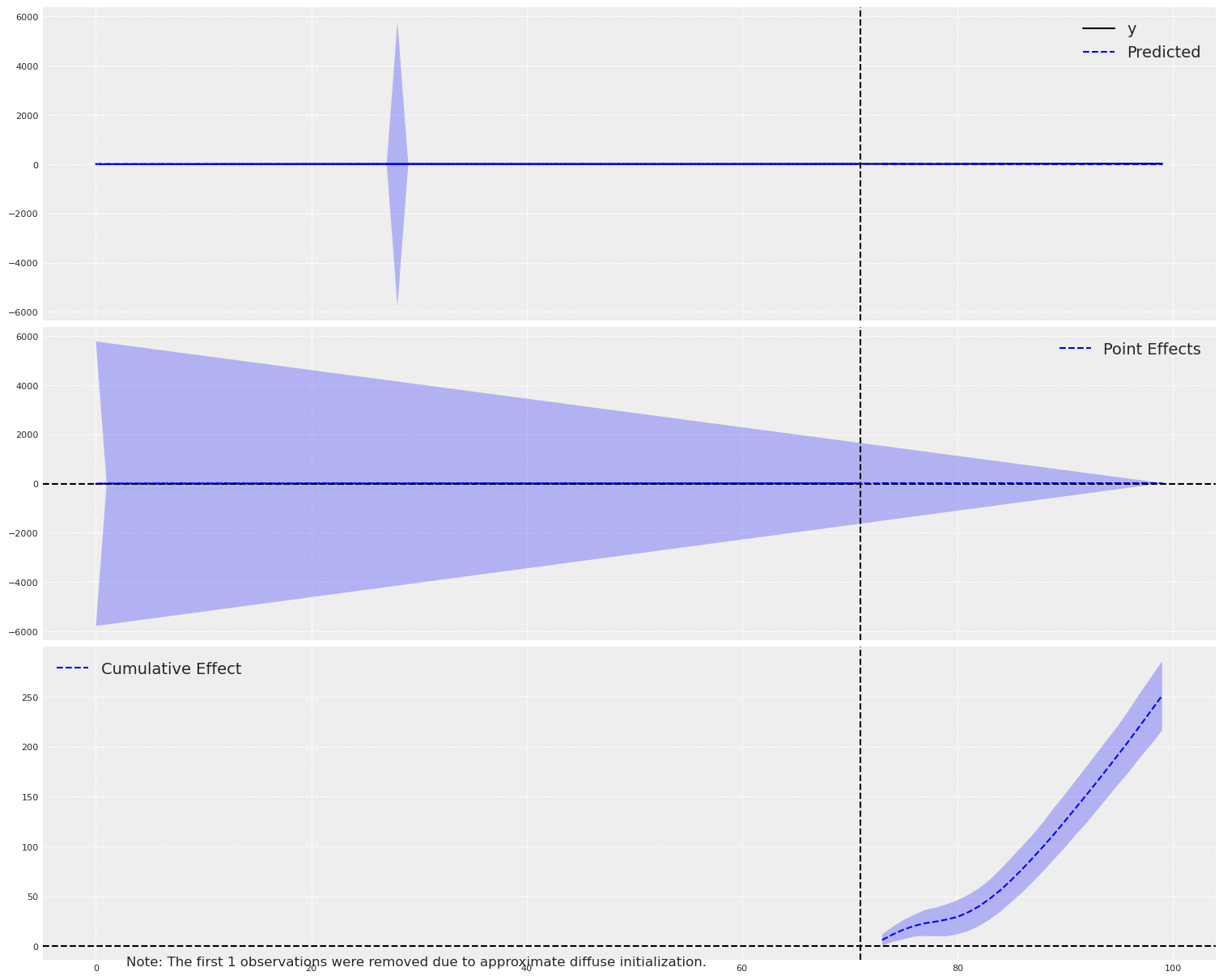
CausalPy’s ITS with the state-space model produces an average effect of around −5.2. The sign is right this time, but the magnitude overshoots the true effect (≈ −1.85) by roughly a factor of three. Again, the model is extrapolating purely from the treated unit’s own temporal structure, with no cross-sectional information. The level of the treated series is largely determined by a combination of the controls — a structure neither ITS method can see, let alone use.
Both CausalImpact and CausalPy’s ITS have now been asked to answer the same question, and both have given different wrong answers. The right question at this point isn’t “which of these is the better ITS implementation?” — it’s is ITS the right method for this data at all?
Why ITS is the Wrong Tool Here#
Let’s pause and think about what we just did. In both CausalImpact and CausalPy’s ITS, we modeled the treated unit’s time series and projected a counterfactual forward. Both methods relied only on the treated unit’s own history — CausalImpact with a BSTS framework, and CausalPy’s ITS with a structural state-space decomposition (level, trend, and — here, nominally — seasonal components). Neither used the control units.
But look at the data again. We have seven control units that were not affected by the intervention. These aren’t just covariates to throw into a regression — they’re donor units that can be combined to construct a synthetic version of the treated unit.
This is the fundamental insight of the Synthetic Control method: instead of modeling time, we model the relationship between units. We find a weighted combination of control units that closely matches the treated unit in the pre-intervention period, and then we use that same combination to project what the treated unit would have done without the intervention.
Important
The key difference
ITS asks: “Given the treated unit’s own history, what would it have done next?”
Synthetic Control asks: “Given how control units behave, what combination of them best approximates the treated unit?”
When you have multiple unaffected control units, Synthetic Control exploits richer information. ITS ignores it.
The problem with ITS here is subtle but important: we’re asking a single time series model to extrapolate forward, relying only on the temporal structure of the treated unit itself. Any trend break, seasonality shift, or structural change in the post-period could be misattributed to the intervention. With Synthetic Control, we have a concurrent control group — the counterfactual moves with the controls in real time, not from a projection.
“But what if I add covariates to ITS?”#
A natural objection at this point: couldn’t we just add the control units as covariates to CausalImpact and fix the problem? After all, CausalImpact does accept covariates — it would use the control units as predictors in its BSTS regression component.
This is actually a real technique called Comparative Interrupted Time Series (CITS) [Lopez Bernal et al., 2018], and CausalPy supports it too. In CITS, you include control units as predictors in your ITS formula (e.g., treatment ~ 1 + control), which helps account for common trends and external shocks that affect both treated and control units simultaneously.
But even CITS has important limitations compared to Synthetic Control:
Aspect |
ITS |
CITS |
Synthetic Control |
|---|---|---|---|
Control units |
None |
Yes, as predictors |
Yes, as donors |
Weight constraint |
N/A |
None (unconstrained regression) |
Sum to 1 (convex combination) |
Interpretation |
Counterfactual from time trends |
Counterfactual from controls + trends |
Weighted combination of controls |
Intercept |
Typically yes |
Yes |
Typically no |
The key differences matter:
CITS treats controls as regression predictors with unconstrained coefficients and an intercept. This means the model can extrapolate outside the observed range of the controls — a source of potential bias.
Synthetic Control constructs a convex combination of donors (weights sum to 1, non-negative) [Abadie et al., 2010]. This forces the counterfactual to stay within the “envelope” of the controls, which is more principled when the treated unit is genuinely a mixture of the control units.
CITS is vulnerable to control unit contamination — if the intervention indirectly affects the controls, the counterfactual will be biased.
In short, CITS is a real improvement over pure ITS, and sometimes it’s exactly the right tool. But it’s not Synthetic Control, and the two methods make fundamentally different assumptions.
Want to go deeper?#
CausalPy supports Comparative ITS out of the box. See the Comparative ITS notebook for a full worked example using a geo-experimentation scenario, including how to check parallel trends, interpret model coefficients, and diagnose model convergence.
The Flexibility Problem#
Here’s where things get interesting from a tooling perspective.
You’ve just realized that Synthetic Control is the right method for this data. What do you do?
If you’re using CausalImpact: you’re stuck. CausalImpact only does BSTS-based ITS. Sure, it can include covariates, but it can’t do Synthetic Control. You’d need to find a completely different package, learn a different API, reformat your data, and start over.
If you’re using CausalPy: you just change the method call. Same data. Same library. Different method. And if you want to try CITS as a middle ground along the way? That’s a formula change away too.
Let’s see this in action.
The Right Approach: CausalPy’s Synthetic Control#
sc_result = cp.SyntheticControl(
    df,
    treatment_time,
    control_units=control_units,
    treated_units=[treated_unit],
    model=cp.pymc_models.WeightedSumFitter(sample_kwargs=sampler_kwargs),
)
Initializing NUTS using jitter+adapt_diag...
Multiprocess sampling (4 chains in 4 jobs)
NUTS: [beta, y_hat_sigma]
Sampling 4 chains for 1_000 tune and 550 draw iterations (4_000 + 2_200 draws total) took 5 seconds.
The effective sample size per chain is smaller than 100 for some parameters.  A higher number is needed for reliable rhat and ess computation. See https://arxiv.org/abs/1903.08008 for details
Sampling: [beta, y_hat, y_hat_sigma]
Sampling: [y_hat]
Sampling: [y_hat]
Sampling: [y_hat]
Sampling: [y_hat]
fig, ax = sc_result.plot(plot_predictors=True)
plt.show()
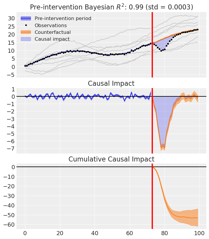
Look at that fit. The synthetic control (the weighted combination of donor units) tracks the treated unit nearly perfectly in the pre-intervention period. After the intervention, we see a clear, clean separation — that’s our causal effect estimate.
Let’s see the summary statistics.
sc_result.summary()
================================SyntheticControl================================
Control units: ['a', 'b', 'c', 'd', 'e', 'f', 'g']
Treated unit: actual
Model coefficients:
    a            0.33, 94% HDI [0.29, 0.37]
    b            0.055, 94% HDI [0.019, 0.09]
    c            0.3, 94% HDI [0.25, 0.34]
    d            0.05, 94% HDI [0.012, 0.089]
    e            0.021, 94% HDI [0.00078, 0.057]
    f            0.2, 94% HDI [0.12, 0.27]
    g            0.043, 94% HDI [0.0042, 0.088]
    y_hat_sigma  0.26, 94% HDI [0.22, 0.31]
stats = sc_result.effect_summary(treated_unit=treated_unit)
print(stats.text)
Post-period (73 to 99), the average effect was -1.98 (95% HDI [-2.30, -1.62]), with a posterior probability of an increase of 0.000. The cumulative effect was -53.39 (95% HDI [-62.22, -43.63]); probability of an increase 0.000. Relative to the counterfactual, this equals -10.17% on average (95% HDI [-11.67%, -8.48%]).
Side-by-Side: Three Estimates, One Truth#
Now let’s put it all together. We have three estimates of the causal effect:
CausalImpact (BSTS, no controls)
CausalPy ITS (structural state space, no controls)
CausalPy Synthetic Control (weighted combination of donors)
And we have the ground truth. The figure below shows the per-period causal effect estimate in the post-intervention window (n = 27) for each method. Shaded bands are 95% HDIs; the dashed black line is the known simulated effect. All three panels share y-limits so magnitudes can be compared directly.
# Extract the known ground truth from the dataset
true_effect = df["causal effect"].iloc[treatment_time:].values
n_post = len(true_effect)


def hdi_bounds(da, hdi_prob=0.95):
    """95% HDI per time point. Returns (lower, upper) arrays shaped (n_post,)."""
    samples = da.stack(sample=("chain", "draw")).transpose("obs_ind", "sample").values
    bounds = np.array([az.hdi(row, hdi_prob=hdi_prob) for row in samples])
    return bounds[:, 0], bounds[:, 1]


# CausalImpact: `inferences` already carries pointwise 95% intervals.
ci_inferences = ci.inferences
post_mask = ci_inferences.index >= treatment_time
ci_effect = ci_inferences["point_effects"][post_mask].values
ci_lower = ci_inferences["point_effects_lower"][post_mask].values
ci_upper = ci_inferences["point_effects_upper"][post_mask].values

# CausalPy ITS
its_impact = ssts_result.post_impact.isel(treated_units=0)
its_mean = its_impact.mean(("chain", "draw")).values
its_lower, its_upper = hdi_bounds(its_impact, hdi_prob=0.95)

# CausalPy Synthetic Control
sc_impact = sc_result.post_impact.sel(treated_units=treated_unit)
sc_mean = sc_impact.mean(("chain", "draw")).values
sc_lower, sc_upper = hdi_bounds(sc_impact, hdi_prob=0.95)

fig, axes = plt.subplots(nrows=3, ncols=1, figsize=(10, 10), sharey=True)

panels = [
    (
        axes[0],
        "CausalImpact (BSTS)",
        COLOR_CI,
        ci_effect,
        ci_lower,
        ci_upper,
        "CausalImpact",
    ),
    (
        axes[1],
        "CausalPy ITS (structural state space)",
        COLOR_ITS,
        its_mean,
        its_lower,
        its_upper,
        "CausalPy ITS",
    ),
    (
        axes[2],
        "CausalPy Synthetic Control",
        COLOR_SC,
        sc_mean,
        sc_lower,
        sc_upper,
        "CausalPy SC",
    ),
]

for ax, title, color, mean, lo, hi, label in panels:
    ax.fill_between(range(n_post), lo, hi, alpha=0.2, color=color, label="95% HDI")
    ax.plot(range(n_post), mean, color=color, linewidth=2, label=label)
    ax.plot(
        range(n_post),
        true_effect,
        color="black",
        linewidth=1.5,
        linestyle="--",
        label="True effect",
        zorder=10,
    )
    ax.axhline(y=0, color="grey", linestyle=":", alpha=0.5)
    ax.set(title=title, ylabel="Causal Effect")
    ax.legend(fontsize=8, loc="best")

axes[-1].set_xlabel("Post-intervention period")
fig.suptitle("Effect Estimation: Three Methods, One Ground Truth", fontsize=14)
plt.show()
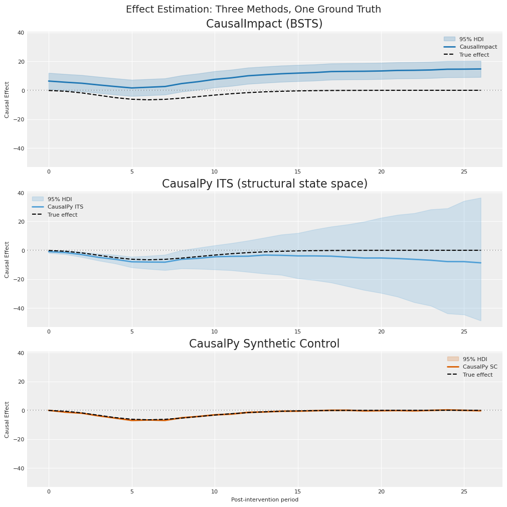
The figure makes the pedagogical point directly:
CausalImpact (top panel) estimates a large positive effect (≈ +9.3) when the truth is negative (≈ −1.85). With no access to the controls, its BSTS model extrapolates the pre-period level and trend and reads the post-period gap as a treatment effect.
CausalPy ITS (middle panel) gets the direction right (negative) but overshoots the magnitude by roughly 3×, estimating ≈ −5.2. A structural state-space decomposition of the treated series alone still cannot see that the series’ level is driven by the control units.
CausalPy Synthetic Control (bottom panel) tracks the true effect curve closely (≈ −1.98 against truth ≈ −1.85), because its counterfactual is built from the donor pool rather than extrapolated from the treated series.
Let’s quantify the differences:
# Compute mean absolute error for each method
mae_ci = np.mean(np.abs(ci_effect - true_effect))
mae_its = np.mean(np.abs(its_mean - true_effect))
mae_sc = np.mean(np.abs(sc_mean - true_effect))

print(f"{'Method':<42} {'Mean Abs Error':>15} {'Avg Effect':>12} {'True Avg':>10}")
print("-" * 82)
print(
    f"{'CausalImpact (BSTS)':<42} {mae_ci:>15.3f} {ci_effect.mean():>12.3f} {true_effect.mean():>10.3f}"
)
print(
    f"{'CausalPy ITS (structural state space)':<42} {mae_its:>15.3f} {its_mean.mean():>12.3f} {true_effect.mean():>10.3f}"
)
print(
    f"{'CausalPy SC (Synthetic Control)':<42} {mae_sc:>15.3f} {sc_mean.mean():>12.3f} {true_effect.mean():>10.3f}"
)
Method                                      Mean Abs Error   Avg Effect   True Avg
----------------------------------------------------------------------------------
CausalImpact (BSTS)                                 11.151        9.299     -1.851
CausalPy ITS (structural state space)                3.445       -5.296     -1.851
CausalPy SC (Synthetic Control)                      0.240       -1.977     -1.851
The numbers make two separate claims that are worth keeping distinct:
Method selection. Synthetic control is the right method for this data structure, because the treated unit’s pre-period level is largely determined by a combination of the controls. Both ITS-family methods, denied access to that cross-sectional information, extrapolate the treated series and mis-attribute the level gap to the intervention. The MAE gap here (SC ≈ 14× lower than CausalPy ITS, ≈ 46× lower than CausalImpact) is primarily a method gap, not a library gap — a well-tuned CITS with these controls would recover most of the ground that ITS lost.
Framework flexibility. CausalPy happens to let you switch methods without leaving the framework. Same dataset, same Bayesian infrastructure, a different class —
InterruptedTimeSeries,ComparativeInterruptedTimeSeries,SyntheticControl. That matters practically: when a first attempt at a method reveals the data wants a different one, you do not have to port your workflow to a new package.
What We’ve Learned#
Method selection matters more than tool sophistication. A well-engineered implementation of the wrong method still answers the wrong question.
ITS is not wrong — it’s limited. When you only have a single treated series and no plausible donor pool, ITS is exactly what you need. When donors are available, synthetic control exploits strictly more information.
The right counterfactual comes from the right model. A counterfactual built from concurrent controls generally outperforms one built from temporal extrapolation alone — when the data supports it.
Before reaching for an ITS tool on your own problem, ask#
Do I have other units that plausibly did not receive the intervention, and whose pre-period series are a reasonable mixture basis for my treated unit? (If yes → SC or CITS is in play.)
Is my treated unit’s pre-period behaviour driven more by shared time trends across units (→ SC / CITS) or by its own internal structure such as seasonality and level (→ ITS)?
Could the intervention spill over into the candidate controls? If so, neither CITS nor SC is clean, and the question becomes one of finding uncontaminated donors.
Example to work through. A retailer launches a new loyalty scheme in one region. The other regions run the old scheme and are observed weekly. Which method fits — ITS, CITS, or synthetic control? (Hint: it depends on whether the other regions are plausibly unaffected, and on how much of the treated region’s pre-period behaviour is explained by the other regions versus its own level and trend.)
Tip
CausalPy also supports Difference-in-Differences, Regression Discontinuity, Regression Kink, and Inverse Propensity Weighting — all within a unified Bayesian framework. The method should follow from the data and the research question.
%load_ext watermark
%watermark -n -u -v -iv -w -p causalpy,pymc,arviz
Last updated: Thu, 16 Apr 2026

Python implementation: CPython
Python version       : 3.13.9
IPython version      : 9.7.0

causalpy: 0.8.0
pymc    : 5.26.1
arviz   : 0.22.0

arviz       : 0.22.0
causalimpact: 0.1.1
causalpy    : 0.8.0
matplotlib  : 3.10.8
numpy       : 2.3.5
pandas      : 2.3.3
seaborn     : 0.13.2

Watermark: 2.6.0